From N to Standard Deviation
This post goes back and forth between computing statistics for a single variable and visualizing these values. I’m using a subset of the gapminder dataset — European countries in 2007, and focusing on the Life Expectancy variable.
This post is developed from lecture slides for my great students in my intro to data science and statistics course at TU Dresden.
I’m most excited about the walk-through of the variance calculation. In preparing to lecture on univariate stats, I came across a nice visualization of variance explained but couldn’t find a visualization just focused on explaining the variance itself. So I made one with ggplot(). You’ll find it in the second half of the post! (I’m going back and forth about whether to include to the code for the plots or not.)
So first we load the tidyverse, which will load ggplot for data visualization and dplyr which we’ll use for data manipulation.
library(tidyverse)
library(gapminder)
gapminder_2007_europe <-
  gapminder %>%
  filter(year == 2007) %>%
  filter(continent == "Europe")
Now I prep a very basic plot. It several lines of code, but most of it is styling; you can actually get away with just the first three lines.
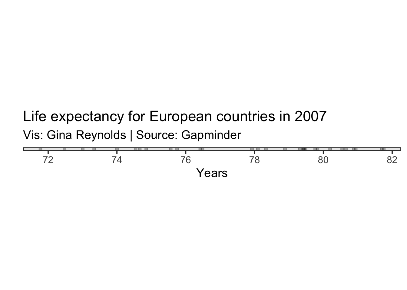
N
You can count the number of observations in your data set using the function, nrow().
nrow(gapminder_2007_europe)## [1] 30Below is one way to tally the number of observations that are missing (NA) in the variable.
# how many missing?
sum(is.na(gapminder_2007_europe$lifeExp))
## [1] 0# how many not missing?
sum(!is.na(gapminder_2007_europe$lifeExp))## [1] 30Measures of Central Tendancy
Mean
The mean is the sum of the values of a variable divided by the number of values. It is a measure of “central tendancy.”
The mean can also be thought of as a balancing point. It the point that, if the folcrum of a balance, with weights of of equal weight at each of the values of the observations, would result in a balanced scale.
\[ \mu = \frac{\sum_{i=1}^{n}x_i}{n} \] In R you can use the mean function to compute this value.
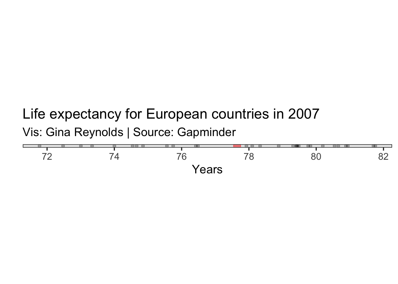
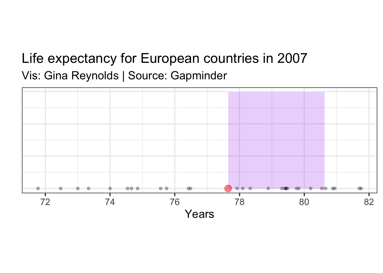
mean(gapminder_2007_europe$lifeExp)## [1] 77.6486In the following plot, the mean is plotted in red.

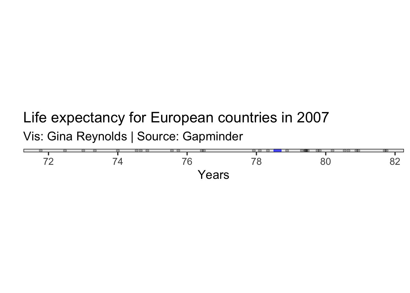
Measures of Central Tendency: Median
Another measure of centrality is the median. The median is the value that has the central position when all the values of are arranged in order.
In R you can comute the median with the function, median().
median(gapminder_2007_europe$lifeExp)## [1] 78.6085In the following plot, the median is shown in blue.
Measures of spread
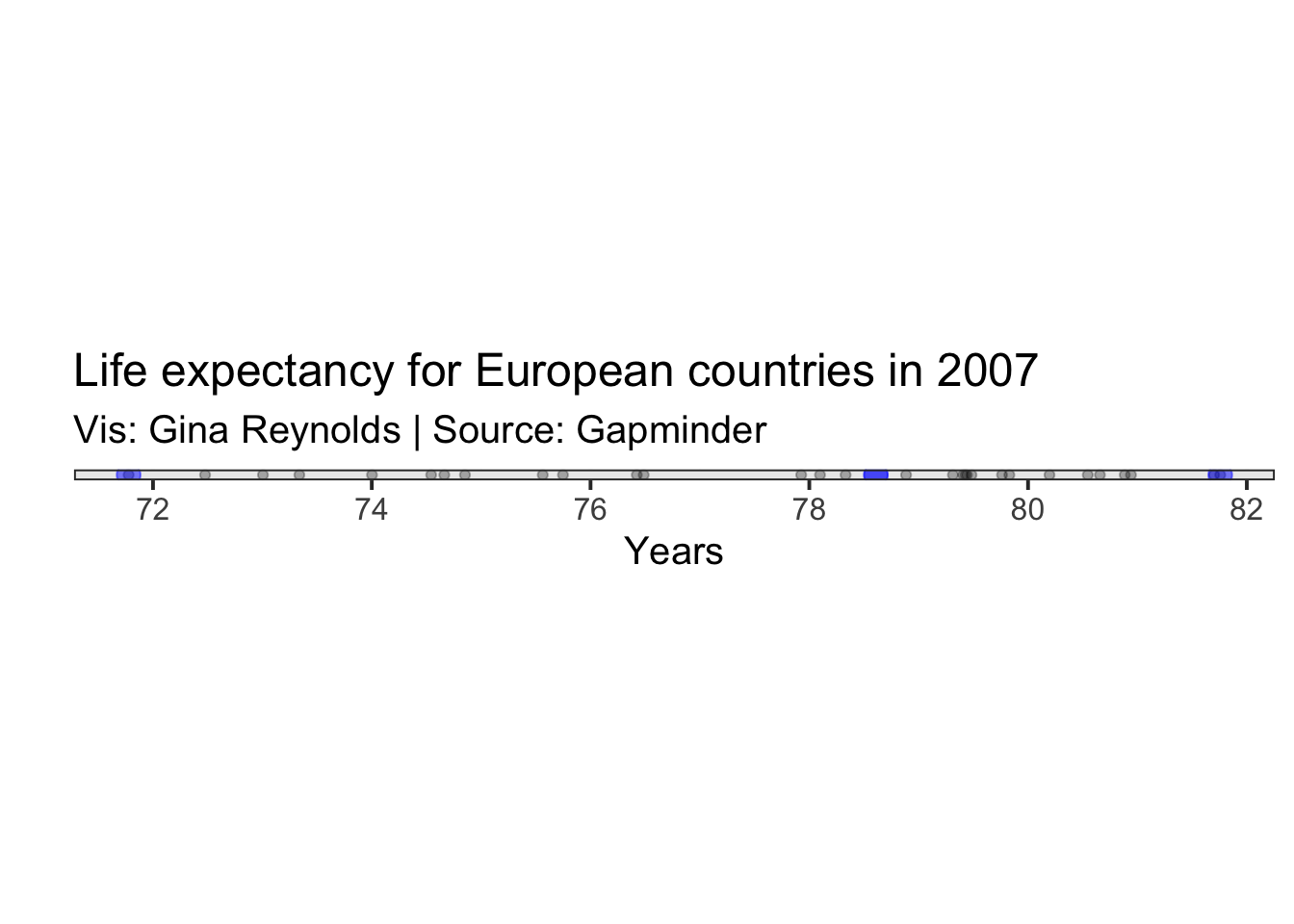
Range
The function range() will return the min and max of a variable.
range(gapminder_2007_europe$lifeExp)## [1] 71.777 81.757I add the min and max on the plot.
Measures of spread/distribution
Range + Median + Innerquartile Range
To find the value at the lower and upper quartile of the data, I usually use quantile, which the argument probs set equal to .25 and .75.
quantile(gapminder_2007_europe$lifeExp,
         probs = c(.25,.75))
## 25% 75%
## 75.02975 79.81225
Communicating spread/distribution
Boxplot
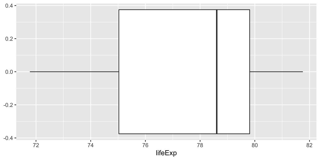
Measure of spread
Variance
\(\sigma^2 = \frac{\sum_{i=1}^{n}(x_i - \mu)^2} {n}\)
You can also use summary to calculate all of these things at once.
summary(gapminder_2007_europe$lifeExp)## Min. 1st Qu. Median Mean 3rd Qu. Max.
## 71.78 75.03 78.61 77.65 79.81 81.76Summary can be used on an entire dataframe too.
summary(gapminder_2007_europe)## country continent year lifeExp
## Albania : 1 Africa : 0 Min. :2007 Min. :71.78
## Austria : 1 Americas: 0 1st Qu.:2007 1st Qu.:75.03
## Belgium : 1 Asia : 0 Median :2007 Median :78.61
## Bosnia and Herzegovina: 1 Europe :30 Mean :2007 Mean :77.65
## Bulgaria : 1 Oceania : 0 3rd Qu.:2007 3rd Qu.:79.81
## Croatia : 1 Max. :2007 Max. :81.76
## (Other) :24
## pop gdpPercap
## Min. : 301931 Min. : 5937
## 1st Qu.: 4780560 1st Qu.:14812
## Median : 9493598 Median :28054
## Mean :19536618 Mean :25054
## 3rd Qu.:20849695 3rd Qu.:33818
## Max. :82400996 Max. :49357
## Variance: Visual walk through
Now let’s walk through this formula piece by piece. First we need the mean.
Variance: \(\sigma^2 = \frac{\sum_{i=1}^{n}(x_i - \mu)^2} {n}\)
Then we do an operation for each of our observations. Take the difference of the value for the observation and square it. Let’s just do that for one of our observations. Romania sounds good. We plot it in green.
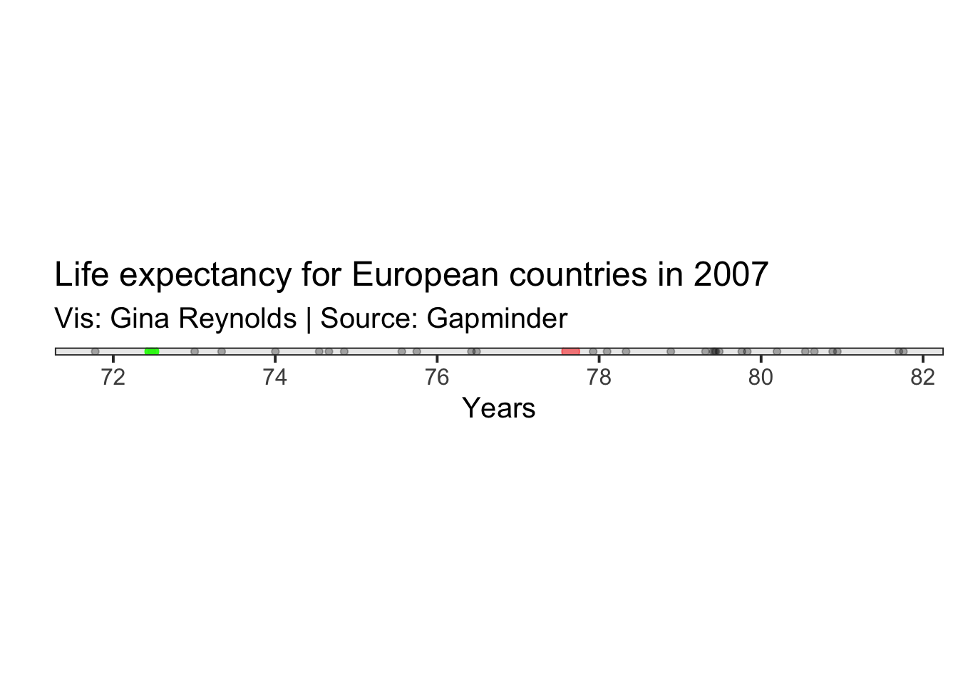
The difference between and the life expectancy for Romania is represented by a distance in our graph. This difference is shown as a green line.
Variance: \[ \sigma^2 = \frac{\sum_{i=1}^{n}(x_i - \mu)^2} {n}\] Calculation for Romania: \[ (x_{Romania} - \mu) \]
## Warning: Use of `gapminder_2007_europe$lifeExp` is discouraged. Use `lifeExp`
## instead.
Variance: \[ \sigma^2 = \frac{\sum_{i=1}^{n}(x_i - \mu)^2} {n} \]
Then we need to square that difference. This resultant value is equal to the area of a square that has the length of the distance between of our life expectancy for Romania and the mean life expectancy. It is a transparent green square in the plot.
Calculation for Romania: \((x_{Romania} - \mu)^2\)
## Warning: Use of `gapminder_2007_europe$lifeExp` is discouraged. Use `lifeExp`
## instead.

## Warning: Use of `gapminder_2007_europe$lifeExp` is discouraged. Use `lifeExp`
## instead.

## Warning: Use of `gapminder_2007_europe$lifeExp` is discouraged. Use `lifeExp`
## instead.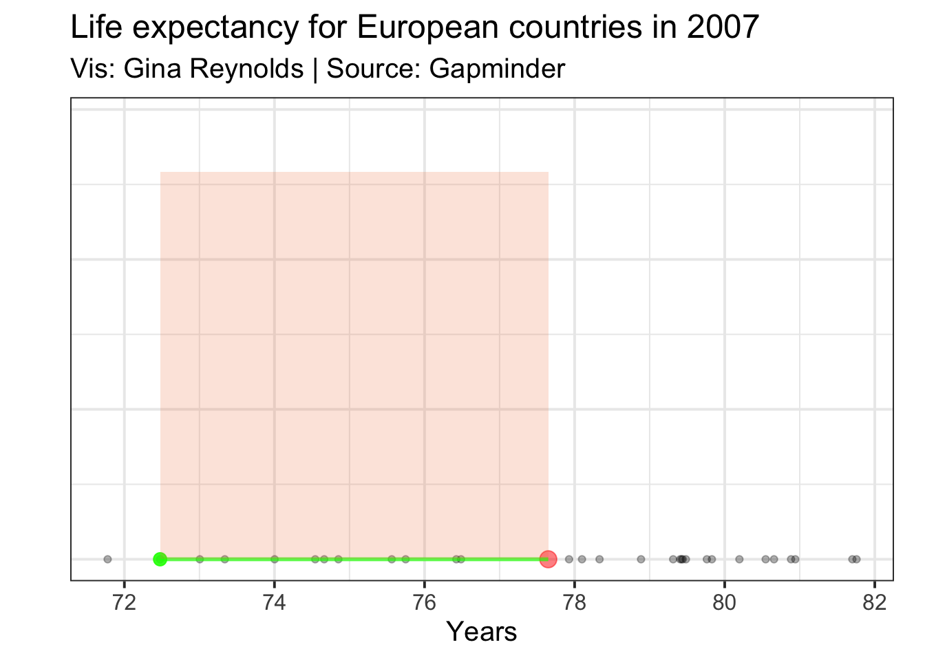
Variance: \[ \sigma^2 = \frac{\sum_{i=1}^{n}(x_i - \mu)^2} {n} \]
Now we need to do the same for all of our observations. Not just Romania, but also Germany, Italy, Sweden, France, and so on.
## Warning: Use of `gapminder_2007_europe$lifeExp` is discouraged. Use `lifeExp`
## instead.

## Warning: Use of `gapminder_2007_europe$lifeExp` is discouraged. Use `lifeExp`
## instead.

## Warning: Use of `gapminder_2007_europe$lifeExp` is discouraged. Use `lifeExp`
## instead.

## Warning: Use of `gapminder_2007_europe$lifeExp` is discouraged. Use `lifeExp`
## instead.

## Warning: Use of `gapminder_2007_europe$lifeExp` is discouraged. Use `lifeExp`
## instead.

## Warning: Use of `gapminder_2007_europe$lifeExp` is discouraged. Use `lifeExp`
## instead.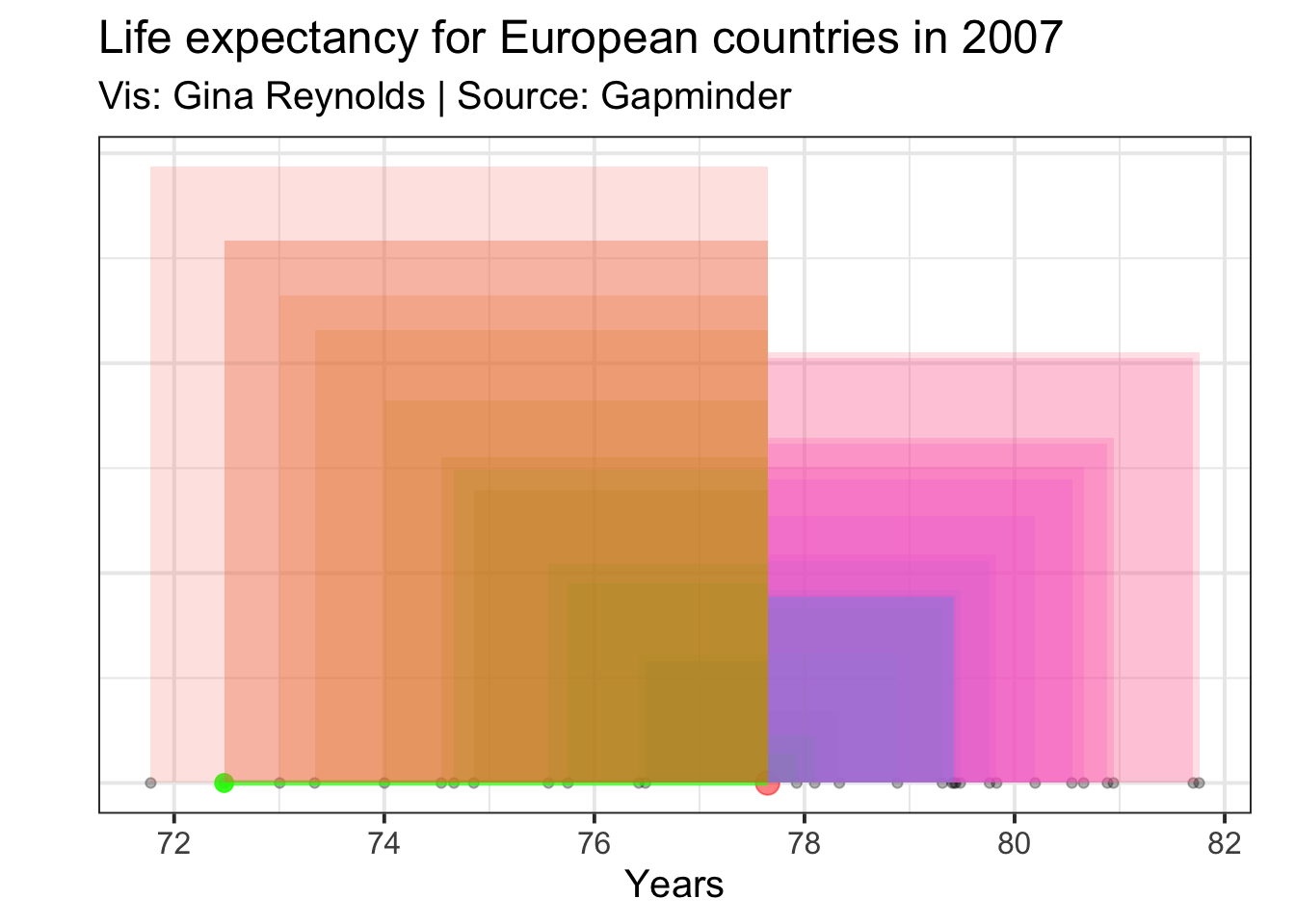
The mean for these areas is the variance.
We sum up all of the resulting areas that are shown in the plot (note that these are overlapping):
\[ \sum_{i=1}^{n}(x_i - \mu)^2 \]
And then we divide through by the number of observations (e.g. the total number of squares) which gives us our aim - the variance, represented as \(\sigma^2\):
\[\sigma^2 = \frac{\sum_{i=1}^{n}(x_i - \mu)^2} {n}\]
I’m plotting the variance as a square where the area is the variance, and a corner of this square (in purple) happens to be at the mean value. The square’s area is the average area for all the squares plotted above, and is equal to the variance.
Standard Deviation:
Now, calculating the standard deviation is straightforward. Take the square root of the variance.
Standard Deviation: \[\sigma = \sqrt\frac{\sum_{i=1}^{n}(x_i - \mu)^2} {n}\]
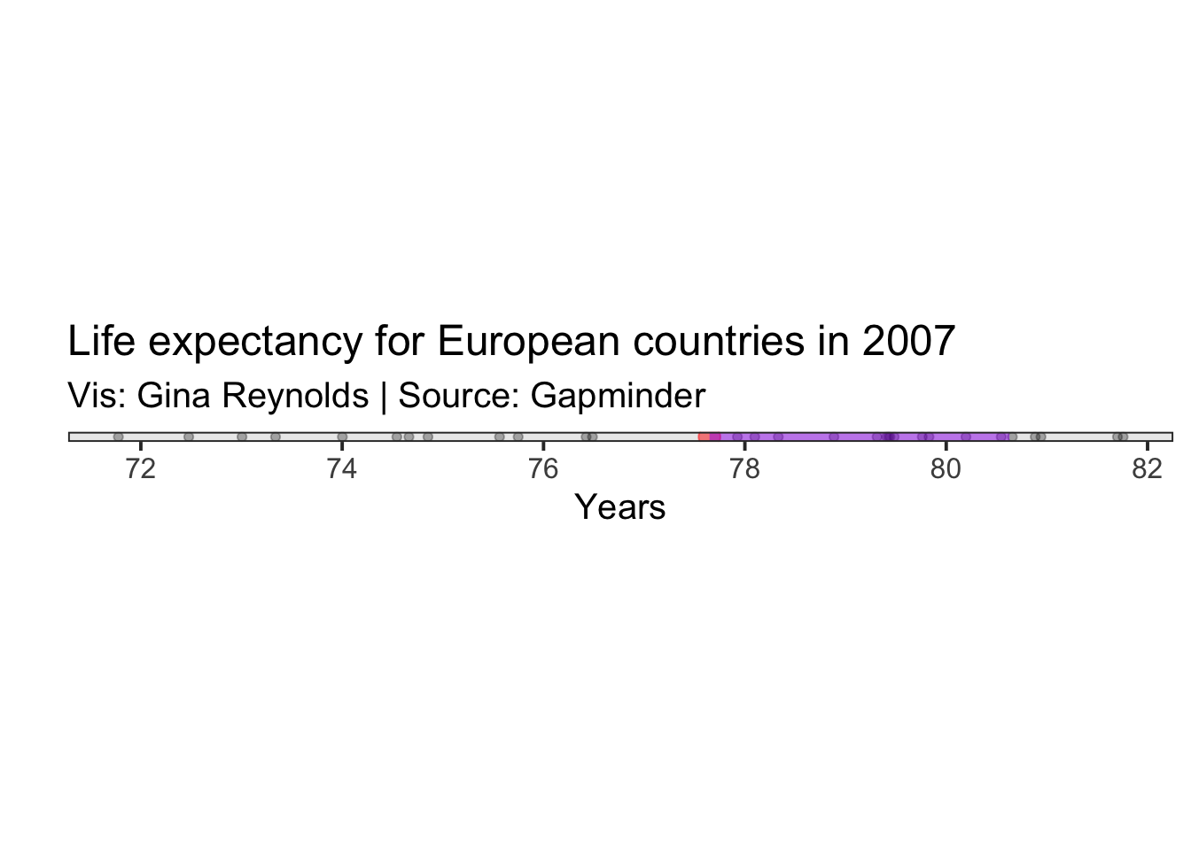
The standard deviation on the plot can be represented as simply the length of the edge of the square whose area is the variance.
Quiz question:
What are the units of each?