Covariance -- A Visual Walk Through
In a previous post, I’ve looked at walking through the calculation of variance and standard deviation, visualizing each step. This post is dedicated to the visualization of another statistic: covariance.
Covariance is a measure of the joint variability of two random variables.
Let’s have a look at the sample covariance equation over all:
\(cov(x,y) = \frac{\sum_{i=1}^n (x_i-\overline{x})(y_i-\overline{y})}{n-1}\)
And now lets apply the equation to the following case:
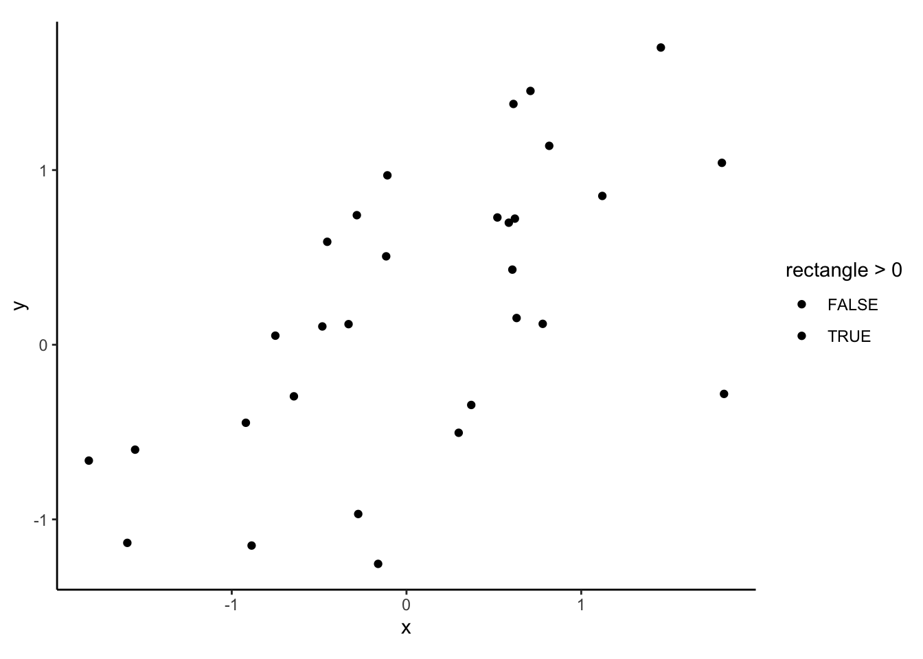
Ready? Okay, now let’s walk through the calculation; there are 7 small steps:
Step 1: find the mean of x:
\(\overline{x}\)
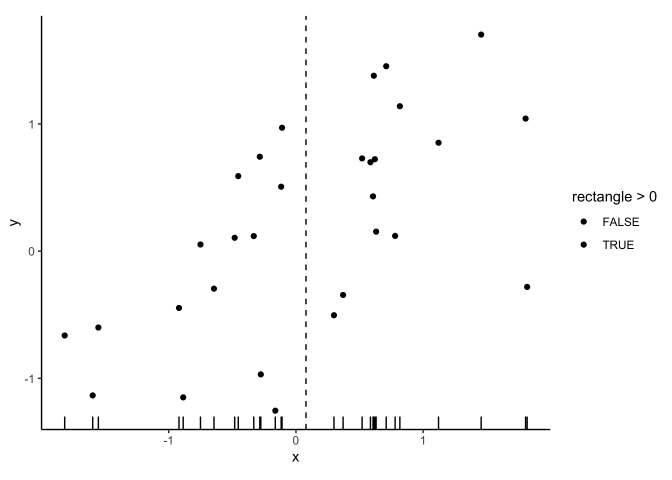
Step 2: find the mean of y
\(\overline{y}\)
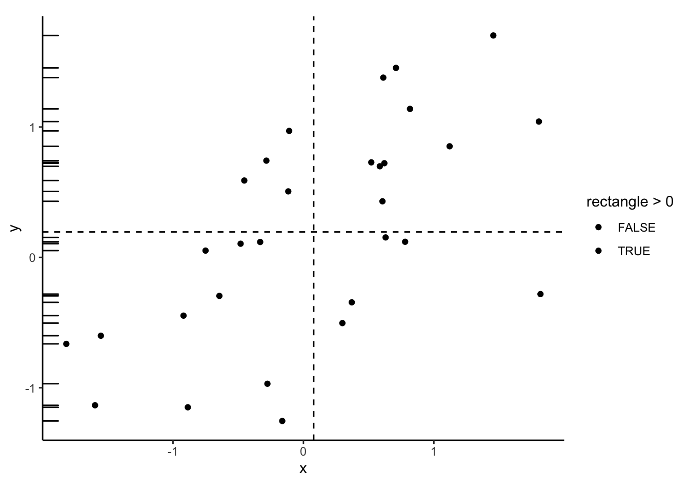
Step 3: calculate difference between x and mean of x
\(x_i-\overline{x}\)
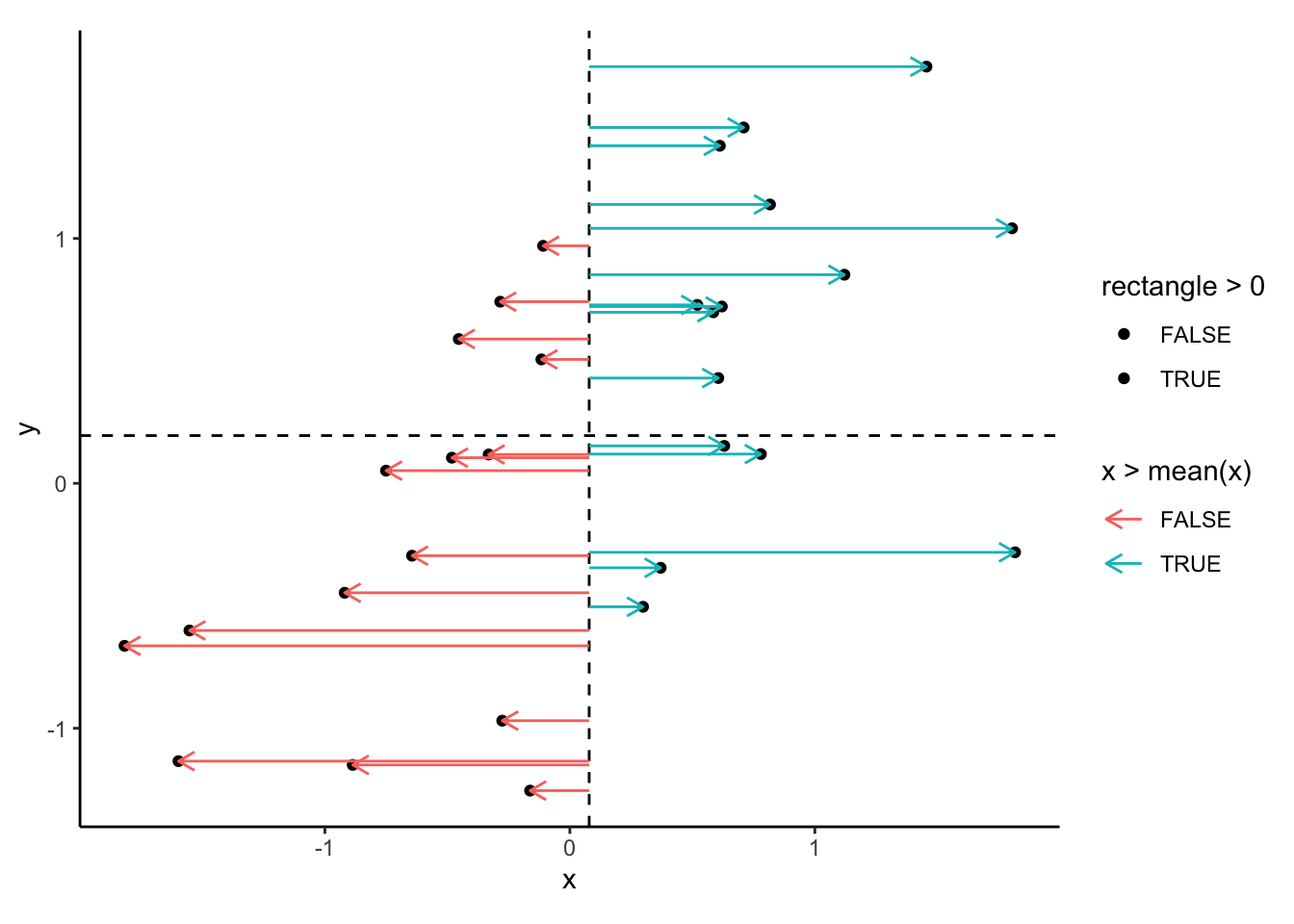
Step 4: calculate difference between y and mean of y
\(y_i-\overline{y}\)
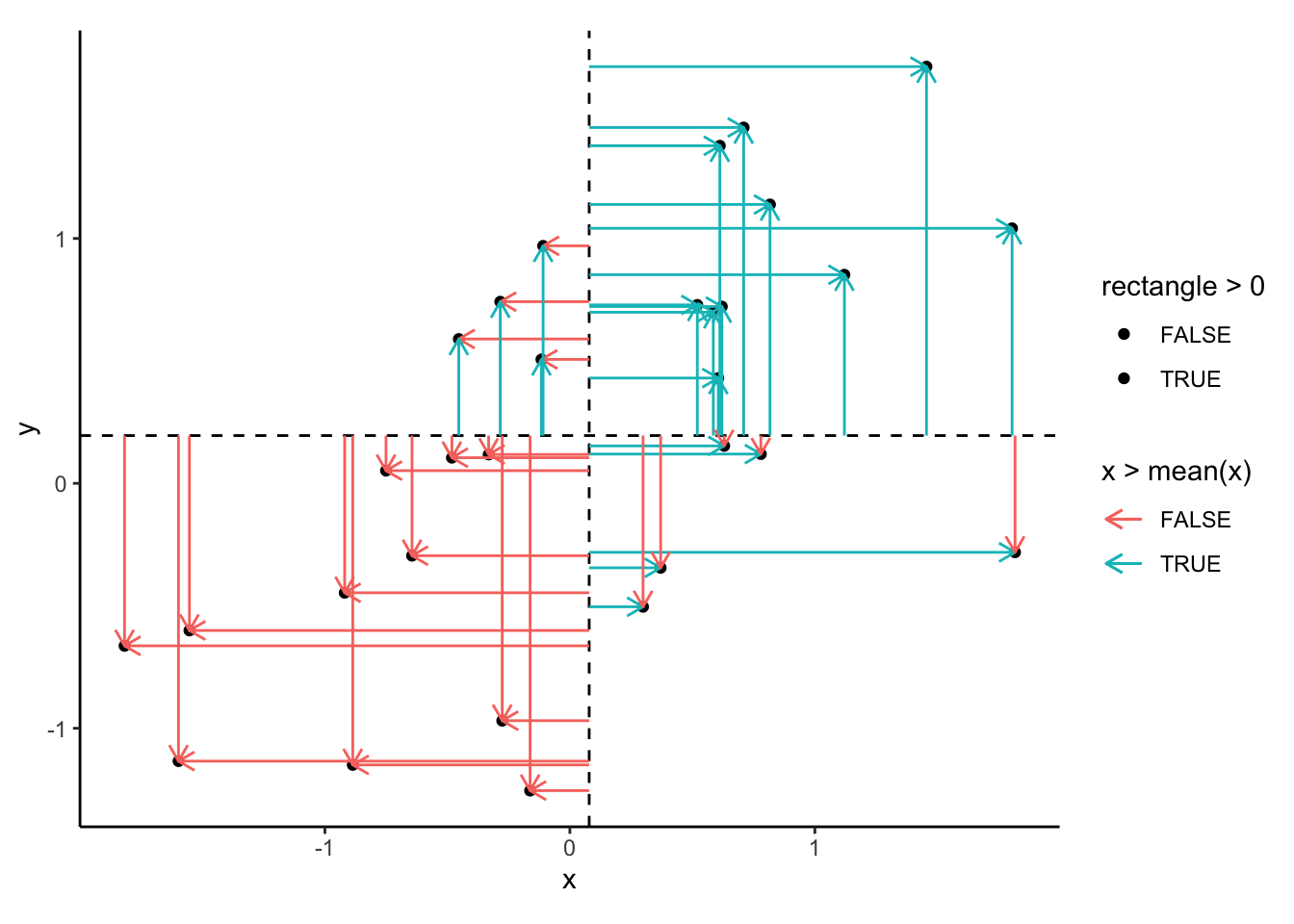
Step 5: multiply these differences (observation-wise)
\((x_i-\overline{x})(y_i-\overline{y})\)
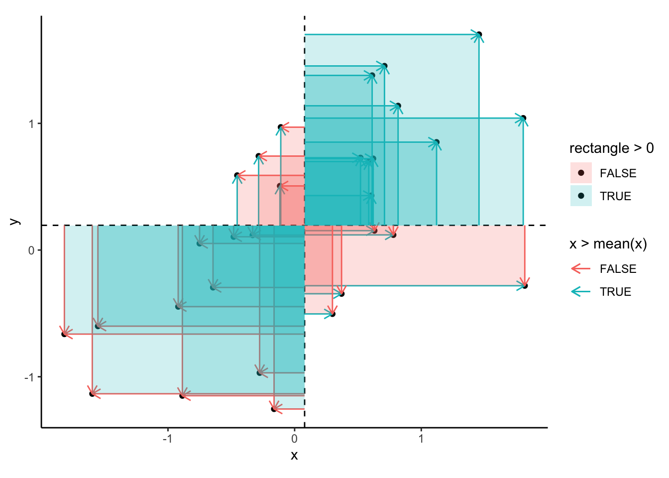
Step 6: Add these areas
\(\sum_1^n (x_i-\overline{x})(y_i-\overline{y})\)
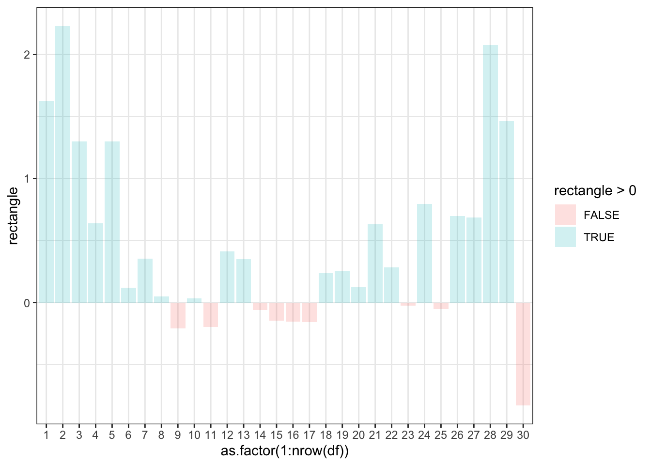
Step 7: Divide through by number of observations minus 1 (the result will a bit larger in magnitude than the average)
\(cov(x,y) = \frac{\sum_{i=1}^n (x_i-\overline{x})(y_i-\overline{y})}{n-1}\)
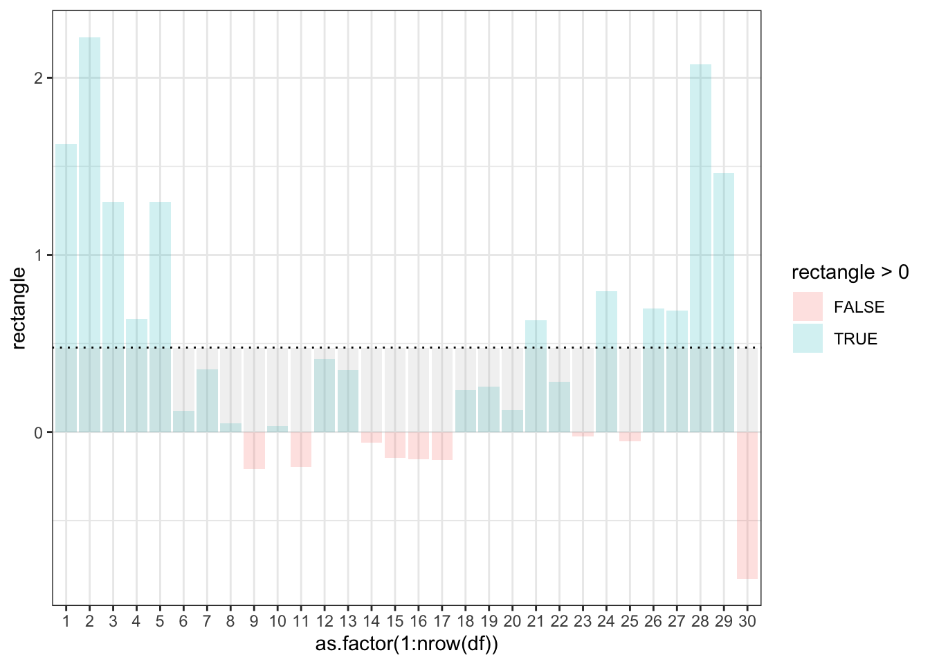
That’s it.
Now we can compare this visualized result to what we would get if we simply trust the R covariance function to calculate this for us.
sum(df$rectangle)/(nrow(df)-1)## [1] 0.4766744cov(x,y) # Calculation for **sample** covariance## [1] 0.4766744Great. It’s a match!
Discussion question
What would the units of unadjusted covariance be for the covariance between life expectancy in years and per capita gdp in dollars?
Note: The normalized version of covariance is Pearson’s correlation coefficient.
References
R Core Team (2018). R: A language and environment for statistical computing. R Foundation for Statistical Computing, Vienna, Austria. URL https://www.R-project.org/.
H. Wickham. ggplot2: Elegant Graphics for Data Analysis. Springer-Verlag New York, 2016.