Central Limit Theorem Demonstration
Sir Francis Galton described the Central Limit Theorem in this way:
I know of scarcely anything so apt to impress the imagination as the wonderful form of cosmic order expressed by the “Law of Frequency of Error”
Why is Sir Francis Galton so excited? Because the Central Limit Theorem (CLT) gives us such clear expectations for random sample means! (A random sample mean is simply the mean of a value for a random sample from a population of interest.) The CLT gives us insight into the question: if we draw a random sample from a population, and calculate the mean for the sample, how close do we expect our sample mean (observed) to be to the true mean (unobserved).
To think about this more, we conduct a thought experiment accompanied by a computational experiment.
The population
In the experiment we’ll be omniscient, but then we’ll think about the perspective of an observer whose knowledge is limited.
As the omniscience being, we will know all about the population and will even create it. Let’s do that now.
x_pop <- runif(10000) # create a popluation with measurable xThe population observations has a feature, x, which we measure for all the units of the population. We can look at the distribution of the variable, and its mean, using the functions hist() and mean().
hist(x_pop) # what does the distribution look like for x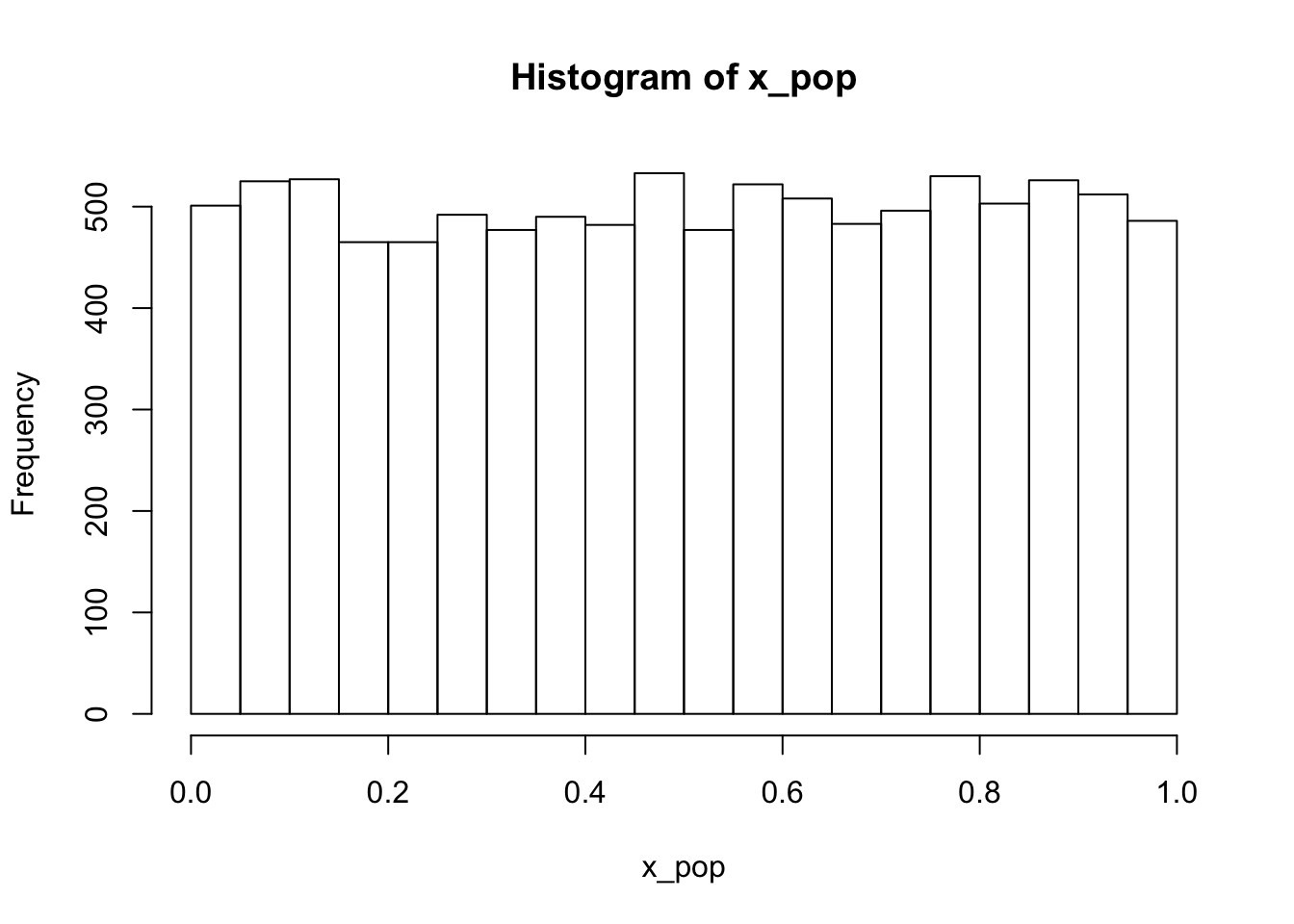
mean(x_pop) # True mean of x (popluation mean)## [1] 0.502301A sample
Now let’s think about the researcher who is not omniscient, but will only observe a random sample from the population. We use the function sample to take a random sample of the population. The population has 100 members, and we sample 30 with the function sample(), which takes a random sample.
x_sample <-
  sample(x = x_pop,
         size = 30)
mean(x_sample) # sample mean
## [1] 0.5342602Interesting. The sample mean for this one sample is not so far from the population mean.
Samples that might have been
In general, how far would we expect the sample mean to be from the population mean? What might we have observed if different samples had been taken?
We are going to use a “for-loop” consider all the samples that might have been taken.
A “for-loop” simply repeats a routine for you, sometimes with different inputs for each time through the routine.
Here is a simple for loop. The loop performs a task (printing “Number:” and the time through the loop) ten times, where the input i changes from 1 to 10.
for(i in 1:10){
print(paste("Number:", i))
}
## [1] "Number: 1"
## [1] "Number: 2"
## [1] "Number: 3"
## [1] "Number: 4"
## [1] "Number: 5"
## [1] "Number: 6"
## [1] "Number: 7"
## [1] "Number: 8"
## [1] "Number: 9"
## [1] "Number: 10"Now back our thought experiment about sampling. What are our expectations about the distribution of sampling means that might be observed for a random sample of the same size?
Let’s repeat the procedure we did above, ten times through. We use the for-loop to do this work for us. We need to use print() in a for-loop to display output.
for(i in 1:10){
  x_sample <- sample(x_pop, 30)
  print(mean(x_sample)) # sample mean
}
## [1] 0.5702718
## [1] 0.4896569
## [1] 0.5011243
## [1] 0.5656035
## [1] 0.4868231
## [1] 0.4608332
## [1] 0.5528666
## [1] 0.4914453
## [1] 0.5719671
## [1] 0.487066Nice! We see 10 different sample means that we might have observed in the case of different random draws of 30 cases! We begin to see a pattern. The means are nearby, sometimes lower, sometimes higher to our true value.
Expectations in the limit
By doing this experiment more times, we can even more precisely illustrate our expectations about where possible sampling means fall in relation to the true population mean.
# Expectations for repeated sampling
all_samples_means <- c() # this vector is an empty container where we will save means
for(i in 1:10000){
  x_sample <- sample(x = x_pop, size = 30)
  all_samples_means[i] <- mean(x_sample) # save the mean for trial i in position i in vector
}
Now we have a vector of sample means that we could have observed, if different samples were realized.
Lets use the hist() function to have a quick look at the distribution of the data.
hist(all_samples_means)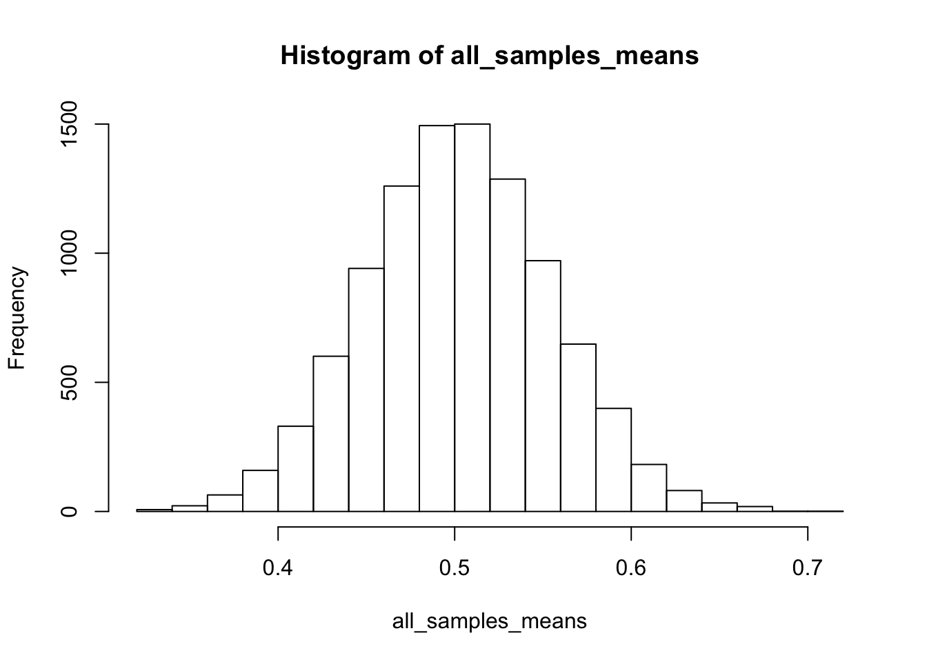
You will notice that the might-have-been-observed sample means are centered around the true population mean. And that these sample means are normally distributed. This regularity is the observation of the Central Limit Theorem that has Galton (and now you?) so excited.
Going further: Other population distributions
What if the distribution in our population looked different? What would the expectation for the distribution of sample means look like?
x_pop <- c(rnorm(400), runif(600))
hist(x_pop)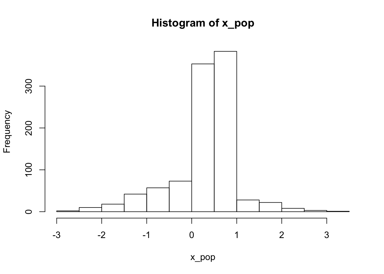
x_pop <- c(rnorm(50,mean = 10), rnorm(50, mean = 5))
hist(x_pop)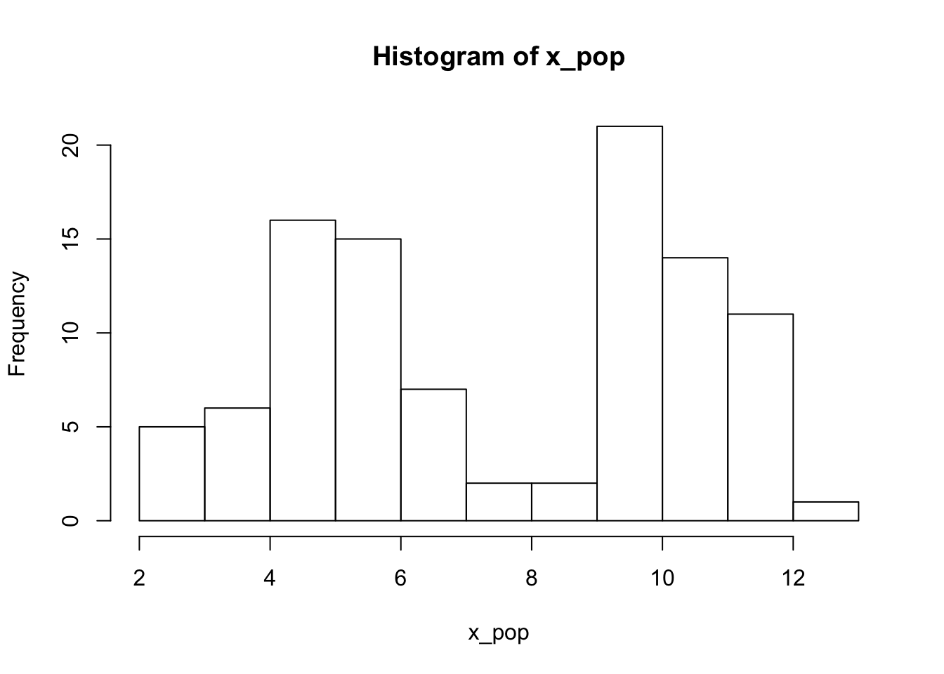
Galton’s quotation continues: Whenever a large sample of chaotic elements are taken in hand and marshalled in the order of their magnitude, an unsuspected and most beautiful form of regularity proves to have been latent all along.
What is the regularity that you find in the results, with different populations as the starting point?